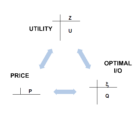
1. Three matrices compose Pareto optimality:
• A utility set [Z,U] describes surfaces of technical indifference for each sector in a model. • A price vector [P] records the efficient price for each commodity. • Optimal rates of physical input/output [x,Q] designate an operating point on each utility surface. |
 |
Gradients of the utility surfaces at the operating points interact with prices such that any commodity’s value of marginal product in any sector will equal that commodity’s price.
When defined in terms of these variables, the Pareto optimum is a highly redundant mathematical system: any two of these variables is sufficient to specify the third.
SFEcon presumes to accomplish all of these computations in mathematically closed-form through our introduction of hyperbolic descriptions of technical indifference. A brief paper on polynomial factoring introduces this claim.
And a more detailed monograph presents all the calculations surrounding static optimality.
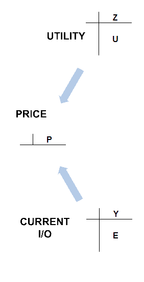
2. SFEcon's dynamics begin with a computation of the physical I/O rates
that are
optimal at current (not necessarily efficient) prices:
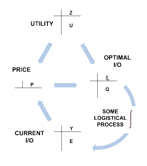
Optimal I/O is then taken as the system’s instantaneous rates of demand. Demand rates drive a process of business logistics whereby physical goods being produced are distributed among the economic sectors where they more or less replace the goods being expended in production. The details of this process are not of critical importance. Model 0’s emulation of business logistics is only to be distinguished as the simplest we can imagine. It is, however, important to note that any operative logistical subassembly must perform a formal integration on demand to establish the levels of each commodity currently in use by each sector. |
 |
Current I/O is to be determined by the current asset levels so that, mathematically speaking, I/O is a delay on optimal I/O; and the state variables by which this delay is accomplished are the physical levels of the sectors’ assets.
For SFEcon, the economy IS a distribution of assets. What the economy DOES is to continuously adjust these asset levels toward their embodiment of general optimality.
3. SFEcon’s Price calculations proceed from the model's continuous awareness of its financial and physical states:
Though not present in the diagram above, it must imagined that demand continuously induces a system of monetary flows to reflect takings of goods off the market at current prices. These monetary flows are integrated into levels of savings and investment that are controlled by flows of interest payments. Monetary levels enter price computations as detailed in the hyperbola monograph cited above. SFEcon’s price computations operate by reference to the current gradients of the utility functions as these are determined by current I/O. These calculations are the same as those by which optimal I/O and utility determine efficient prices. Thus SFEcon presumes that markets value commodities as if their current distribution were optimal — which is no more than to say that markets generate prices so as to motivate the economic system toward the general optimum implicit in its utility parameters. |
 |
4. Putting these conceptual pieces together brings to the closed set of information flows below:
