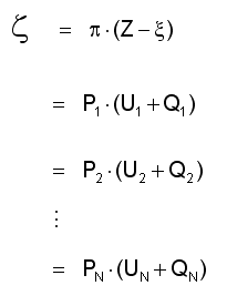
Measures of marginal cost and value begin with a sector’s financial discriminant z $/year, which was developed in connection with our proposed solution to the polynomial factoring problem:

          Eqa. 2-3

If the [p,P_J] set in these equations is taken as holding place for a sector’s marginal cost of production and the marginal values of its inputs J, then marginal costs and values are given by simple functions of a sector’s discriminant z, the shape of its production tradeoffs [Z,U_J], and its current location [x,Q_J] on its production function.

Equation 2-3 presumes that output x and factor usages Q_J are optimal with respect to a set of general equilibrium prices [p,P_J] — a situation that only exists in the abstract, and that no self-respecting theory of economic adjustment would presume to compute. Using the equations of general optimality to represent actual decision-making requires substitutions for z and [x,Q_J] to particularize marginal cost and value equations in terms of an economy’s current state — which states are never optimal and, most importantly, convey no awareness as to where ‘optimal’ might even be.

A sector would of course know is current state [Y,E_J] and use it in substitution for [x,Q_J]. The substitution for z $/year is a bit more interesting in that it must express the sector’s current state without reference to equilibrium money prices [p,P_J]. Equilibrium prices do not exist beyond the abstract realm; but every sector IK certainly has a monetary state expressed in terms of either 1) the dividends -e_IK generated by industrial, profit-making sectors I=1…L-1, or 2) the dividends e_LK received as passive income by household sectors I=L…N. These variables are essentially delays on net cash flows r_IK that were computed from past prices having no reference to equilibria of any kind. A sector’s current e is therefore appropriate in calculating a particularization of z to embody a sector’s current state.

Our investigation of alternate computations for z revealed a variable b referencing the optimal financial services f that -e_IK and -r_IK must come to equal at stasis. Using -e_IK to particularize Equation 7-10 for an industrial sector IK, we arrive at an estimate b for IK’s z that is based entirely on a model’s current (not necessarily equilibrium) state:

Particularization of a household sector LK by reference to Equation 7-14 yields a similar result ...

in which the differences owe their distinction to the contrary nature of the household product.

Model 0 uses the parameters b_IK to infer marginal costs of production MCP and values of marginal product VMP. Substituting a sector JK’s b_JK for z in Equation 2-3’s first equality allows computation of good J’s marginal cost of production MCP $/unit in the currency of economy K:

Substitution of a sector IK’s b_IK for z in Equation 2-3’s other equalities allows inference of sector IK’s marginal valuation VMP $/unit of input J in the currency of economy K:

These equations convey the very stuff of neoclassical causality; but they contain no references in equilibrium, nor to money prices of any calculatory lineage. They express information that is entirely local to a given economic actor, i.e.: his asset levels; the shape of his production tradeoffs; and his financial obligations.