As discussed in connection with Value's Measure, every SFEcon model transacts a zeroth commodity through a zeroth sector. Good J=0 constitutes an artificial financial unit that we have labeled ‘the global currency unit’ GCU, or G. The GCU is a constant value unit insofar as its quantity is always fixed at whatever level it is given at the inception of emulation; and its turnover fraction V₀ is always set at 1/year in recognition of its meaning to the financial computations it supports.

At stasis, sector IK’s flow of value E_I0K G/yr will equal the combined value of its asset flows E_IJK units/year ...

where an asset J’s absolute unit value is given by Y_J G/unit. The sum of all E_I0K over I and K must always equal value’s constant output rate Y₀₀ G/yr

Keeping E_I0K current is accomplished by operation of Model 0’s regular circuit of physical flows. This operation presumes knowledge of: 1) P_0K, the price of one GCU in terms of the currency of an economy K; and 2) asset values Y_J. In this article we will continue our presumption that P_0K is known (it will be determined anon) and proceed here to a express a commodity J's absolute marginal value through the familiar notion of a demand schedule.

We begin with an awareness of IK’s turnover of value E_I0K as known in the manner any asset’s turnover rate E_IJK, viz.: V_J times IK’s stock of J. E_I0K’s significance lies in its value equivalence G/year to a sector IK’s budget constraint s_IK $/year of monies to be expended for asset replenishment:

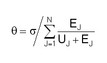
An estimate of what IK needs to expend in order to approach optimality is critical to the analysis because s is the basis of one of our approaches q to an economic sector's financial discriminant z:

       Eqa. 7-5

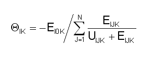
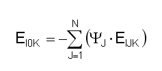
If this equation is to be useful in calculating a global, constant-value commodity prices Y_J G/unit, then we must require that q $/year be expressed as its equivalent in G/year. We hereby introduce Q=q/P_0K as this equivalent. As we are now at a point in the computational cycle prior to our discovery of P_0K, Q must be computed by substituting -E_I0K for s in Equation 7-5: 

Our next reference is to the generic hyperbolic demand schedule:

which we note 1) requires a reference to the financial identities of the sectors I, viz.: z_I, and 2) being limited to a single economy, neglects the subscript K.

Expression of a commodity J's demand schedule for the global sum of all economies K requires attachment of the subscript K=0 to the parameters and independent variables in the above, together with the obvious substitution of Q_IK G/year for all IK’s financial identities z_IK:

Subscript 0 implies that D_J0 is the sum of D_JK over all K=1…M and that U_IJ0 is the sum of U_IJK over all K=1…M. (The second of these sums further implies that the global production function for a sector I can be created by merely adding the production parameters for each J of sector I across all economies K=1…M. Our justification for this procedure is the obvious continuation of an earlier discussion on the peculiar nature of hyperbolic indifference surfaces.)