Measure

SFEcon portrays economic adjustment as a process of sectors IK adjusting asset levels (A_IJK+B_IJK +C_IJK) so that their employments E_IJK =V_J•(A_IJK+B_IJK+C_IJK) of inputs J tend toward optimizing their operations. This process is guided by the sectors’ continuous re-evaluation in terms of their levels of absolute value (A_I0K+B_I0K+C_I0K). Valuation is subject to the requirement that sectors’ turnover of value E_I0K=V₀•(A_I0K+B_I0K+C_I0K) will settle at the sum of products of commodity values Y_J G/unit with physical asset turnovers E_IJK units/year:

And the model’s integrity requires that all of the value flowing at an emulation’s inception Y₀₀ must be kept coursing through the E_I0K’s in their ‘proper’ proportions.

The apportionment of value proceeds via the same circuit of physical flows established among Model 0’s physical rates and levels. Here we see replenishment rates R_IJK driving the circuit by which goods are produced and taken into inventories to more or less replenish that which is extinguished by production. R_IJK was then defined in reference to the current optimal rate Q_IJK for IK to use J:

Eqa. 12-2

Control of physical adjustments was accomplished by setting R_IJK equal to Q_IJK whenever the availability of J is sufficient to do so, and rationing the availability of J according to the proportions of Q_IJK when J is insufficient.

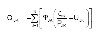
To be operative from the standpoint evaluating the sectors IK, Q_I0K should receive a negative sum on the value equivalents of the demands Q_IJK being expressed in IK’s row:

This is accomplished by redefining Equation 12-2 for the special case of J=0:

The number of z_IK’s in row IK is given by N_IK; Y_J/P_JK has been replaced by 1/P_0K in every term of the sum; and U_I0K is defined as a sum on the values of IK’s utility parameters:

This equation has commodity values Y_J entering the theoretical scheme through the evaluation of U_I0K.

Column zero of our asset replenishment model will then be completed by having the R_I0K’s distribute the entire, invariant supply rate of value units Y₀₀ among the sectors IK in proportion to their Q_I0K’s. (It should be emphasized that full allocation of good 0’s supply Y₀₀ is what keeps the quantity of GCU’s constant; and that this occurs in exception to the practice for all other all other goods, which are left on the market if supply exceeds demand.)

With R_I0K’s known, the reference commodity of value moves through Model 0’s circuit of physical flows in the manner of any physical commodity. The level of value held by a sector IK, i.e.: A_I0K+B_I0K +C_I0K, will be known in just the same fashion as is the level of any physical asset. And the variable E_I0K=V₀•(A_I0K+B_I0K+C_I0K) will continuously re-evaluate the sectors IK in analogy to capitalism’s incessant re-casting of equity values.

With the quanta of value units GCU established for each sector IK, we are poised to compute commodity values Y_J. When the more elusive P_0K’s are also established, Q_I0K’s will be known and the problem of evaluating economic sectors in terms of a constant-value financial unit will have a theoretical solution.