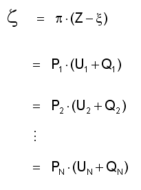
As is the case with an output’s price, its marginal cost of production is expressed as the ratio of a financial quantity to a physical quantity. SFEcon’s hyperbolic system of reference has served-up a variable z $/year as the primary descriptor of economic sector’s financial state; and we proceed here to construct the financial discriminant z as the proper numerator for the ratio describing marginal costs. Equation 2-3 defined z in the course of our discussion on the polynomial factoring problem:

Eqa. 2-3

This equation, being confined to an equilibrium upheld by optimality, allows us to directly identify the price p_J of a sector J’s output with its marginal cost of production at its optimal rate of output x_J:

The equation for marginal cost of production can be re-interpreted as supply schedule for good J upon relaxation of the equilibrium context in which it was derived. We merely identify the optimal output rate x_J as an independent variable rate of supply S_J, presume z_J as known and constant, and accept p_J as the dependent price variable P_J. Insofar as our analysis describes a near-optimum, we have a workable estimate of how price varies with supply:

In the case of the household product of leisure time, the marginal cost of production p_L is negative: the more a household is at leisure, the less its revenue. This condition is effected in that the Z_L of the marginal cost equation is negative and of greater magnitude than x_L, which is also negative. The matter is further complicated in that labor’s supply S_L is a residual of -x_L hours of leisure per year with a labor/leisure sector’s total experience of time t_L:

So: constructing a household supply of labor schedule involves 1) equating the wage P_L with negative sense of marginal cost of leisure p_L, and 2) substituting S_L-t_L for the x in our generic supply schedule: