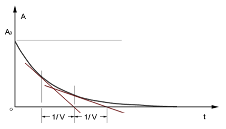
The most primitive naturally-occurring pattern of dynamic adjustment is exponential decay, e.g.: of heat, electrical charge, radioactivity, etc. This pattern can be quite familiar: consider the case of a pizza delivered to a room such that the temperature differential between the pizza and the room equals some amount A₀: left untouched, the pizza’s temperature will drop to that of the room; which corresponds to the temperature differential A decaying away to zero with the passage of time t. According to Newton's curve of cooling, the value of A will vary with t according to the exponential pattern shown below.

Exponential functions are characterized by a unique property: striking a tangent at any point, and extending the tangent to cross the function’s horizontal asymptote will always define the same distance 1/V along the time axis. The functional relation between A and t is given by V and A's initial value A₀:

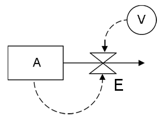
Comparatively few dynamic systems are simple enough to yield closed-form expressions of their behavior such as the equation for exponential decay above. More complicated systems can be made to disclose their dynamics if they can be perceived in terms of a signal path diagram. The signal path for exponential decay, shown below, makes use of the three elements by which all signal paths are composed.

The current level of temperature differential A is depicted by a square. Dissipation of the potential embodied in A is visualized by flow along a solid line leading away from the square. The rate of decay is depicted by a valve symbol attached to the line of flow away from A. Broken lines indicate flows of information, which are considered instantaneous. Thus the instantaneous rate of decay E is always computed by the current level of A, multiplied by the parameter V, which is depicted by a circle. This mechanism indicates that time's passage always has potential A flowing out in proportion to the amount of A that is left. Thus A depletes at the ever-decreasing rates characteristic of exponential decay.

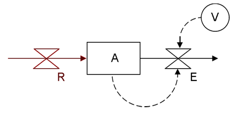
First-order delays are a commonplace of economics where they appear in the form of exponentially-weighted averages. A delay is constructed by attaching an exogenous driving function R to the signal path depicting exponential decay. This driving function carries a series of a data to be averaged.

Whatever pattern is evident in the time-series of R will emerge in attenuated and spread-out form at 1/V time units later in the time-series of E. E is a delay or lag on R; and the current value of E is an exponentially-weighted average on all past values of R. If R is held constant, A will attain a level such that E = V•A = R.

First-order delays have familiar uses in economics and operations analysis. If, for example, R is a series of sales rates for some product, E might disclose appropriate production rates by smoothing the R series. Economists have reference to a certain delay model of consumption and income whereby consumption E is thought to be determined by a lag on income R. This model is considered at some length in SFEcon's treatment of Keynesian economic theory, which we commend as another source of familiarity with the notion of delay.